Intro

In this lab, we’ll be extending the image processing from the previous few labs by adding a convolution module. This will be useful for reducing noise on our masks, but we'll also see that it's useful for detecting other features in our image and...not to be overly dramatic which I know have a tendency to do...can be the foundation of so many important techniques in so many fields.

When you did your masking in weeks 5 and 6, remember how you'd get little clumps of noise around the mask that you'd generate? In our testing, we've found these little extraneous pieces particuarly easy to get with objects that aren't of a matte texture - anything that's shiny or produces a lot of glare is difficult for our cameras to track. Have a look at this:

Here I'm holding up a tasteful red object (that is very Chroma Red and very demure) reasonably far away from the camera, but there's a bunch of speckle noise coming up off the floor and walls, and that's throwing our centroid calculation off. We could fix this by trying to find the largest continuous region of pixels in the image - but this would require some kind of nearest-neighbors approach, and none of those algorithms are "cheap" to implement.

Instead we could attack this by blurring the image before generating the mask - smoothing over the nonuniform parts of our image to get a more consistent blob of color that's easier for us to track. A simple way to do this would be to scan through the image and take the color value of each pixel, and average it with that of it's neighbors. Let's try this on an example image, and we'll average together the 3x3 grid of pixels that surrounds each pixel:

This definitely looks blurred! Blurring isn't always what you want to do, but for this use case, it can help. Once you implement this on your FPGA, you'll see similar results with the image from your camera, and you'll see a reduction in the speckle noise too. This techinque is called convolution, and there's a lot more that you can do with with it than just blurring images. Let's define this in a more rigorous way.

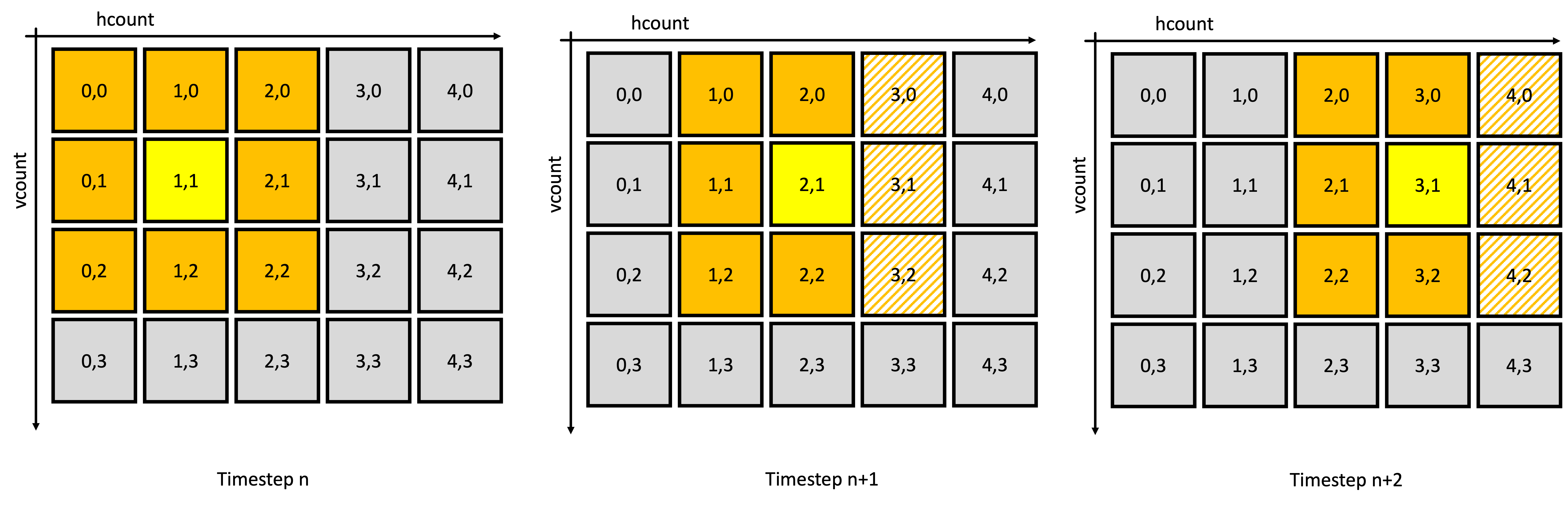
When we did the blurring above, we scanned through each pixel in the image in the left-to-right, top-to-bottom manner that's used in VGA/HDMI/etc. Let's call this pixel our target pixel, shown in yellow below. We took all the pixels in a 3x3 grid around the target pixel, averaged their color channels together, and then set the color of the output pixel to that color. That looked something like this, taken over the whole image:

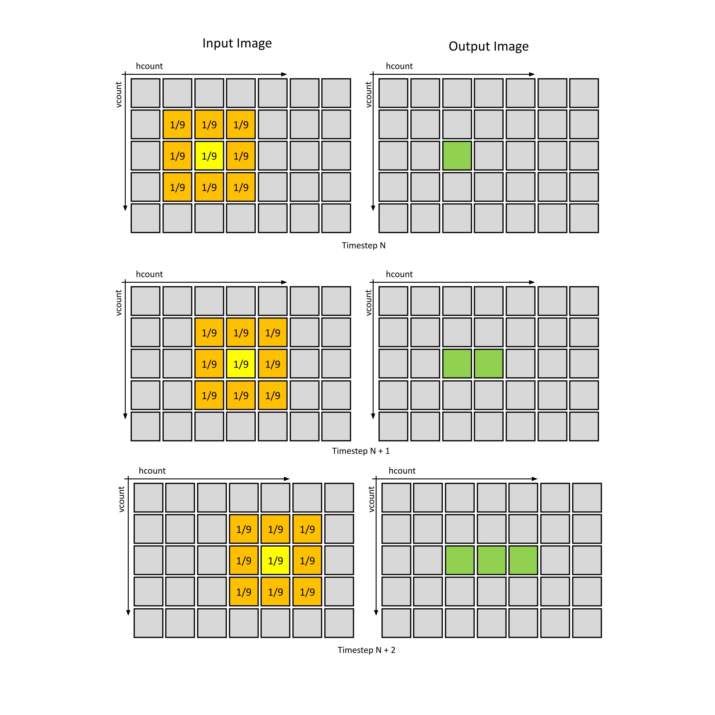
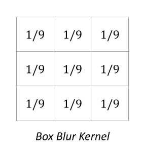
This goes for the entire row, once we hit the end of the row we'll move onto the next one. Another way we could think of this is as dragging a kernel across the input image. The kernel is a matrix which contains the weighting coefficients used in our average. In the case above, each of the 9 pixels got equal share in the output pixel, so each element in our 3x3 kernel was 1/9. Again, we do this for each color channel, not the entire pixel value.

There's a really neat interactive demo of this here if you'd like to play around! This lab will go easier if you have a sense of what we're trying to do here.

Kernels 🌽

We could have just as easily chosen to do the same thing with a differently sized kernel that selected more or fewer pixels, and we also could have changed the weight given to each pixel by the kernel. For example, the kernel for our simple averaging from before could be written as:

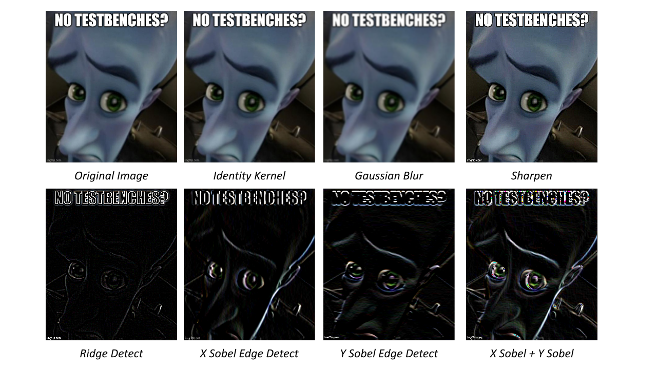
We also have freedom to change the content of the kernel itself, and there's a few that give us some pretty wild effects:

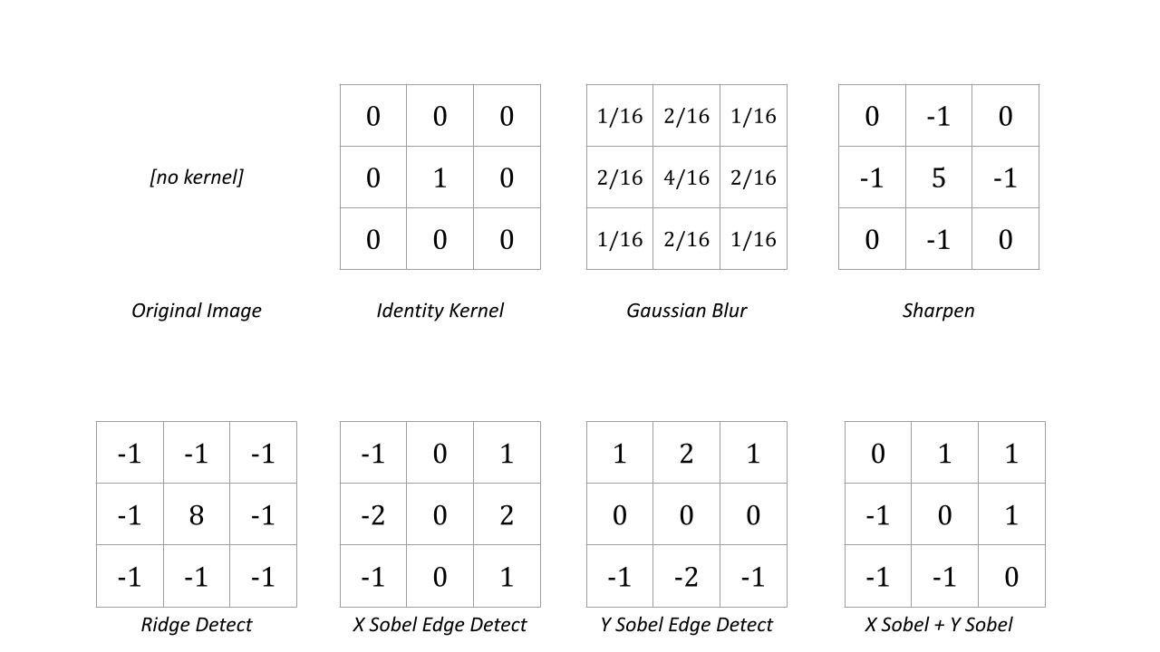
And here's the values of the kernels themselves:

Each of these deserve a little explaination:

• Identity: Arguably the simplest kernel, it just returns the same image when convolved with the input image. Straightforward and a little boring, but we love and cherish it all the same.
• Gaussian Blur: A blur similar to the blur we first introduced, but with weights taken by sampling a 2D gaussian distribution. Since we place more weight on the pixels closer to the center, this has the effect of blurring the image while better preserving the underlying features. Any function that has more weight on the center pixels would do this, but it's pretty common to see the Gaussian used because of it's magical fourier transform properties.
• Sharpen: Accentuates the regions in an image where neighboring pixels have different values. It's actually subtracting a blurred version of the image from the original image.
• Ridge Detection: A kernel that looks for local maxima/minima of a function - similar to a geological ridge, where it gets its name.
• Sobel X and Y Edge Detection: (named after an MIT alum and introduced in the late 1960s). Very similar to sharpen, but we tweak the kernel so that it's preferential towards either the X or Y axis
• X + Y Sobel: Accomplishes edge detection by doing X and Y edge detection on an image, and then taking the vector sum of the results for each pixel. This helps to detect things that don't have their edges lined up exactly along the X and Y axes, and it's what most commonly used in the real world. Here we don't take the vector sum since that's computationally expensive, we just average the two components together.

There's a bunch of other convolutional kernels that are common in image processing (Unsharp Masking, Emboss, the list goes on...and then you can also have variations on these with offsets and things) but we'll start with just these. And as your kernel gets larger and larger (we'll stick with just 3x3 in this lab), you get lots more options. At large enough scales, these kernels basically can start to act like matching filters, scanning for particular patterns in the image...and all the math that goes into this is basically the same that you see in many image-processing neural networks. In fact, the application of kernels to 2D images is essentially what the C part of CNN (Convolutional Neural Nets) is all about, since we are convolving after all.

Getting Started

You'll need all the same hardware from last week - the camera board, something to track on Cr or Cb, an unwavering sense of adventure, etc...

A few new/changed files for the hdl folder are included here. You should use those, but you should also make sure to bring over all other files (From data, etc...) to this project. A slightly modified xdc file to take care of some clock-domain crossing timing issues should also be used.

Because we're using some new features and we're ignoring some old ones, we've got a new top_level.sv file for you. You really shouldn't need to modify this file at all in this lab. Everything should be pre-wired. It is largely based on lab 5, but some switch options with the switches from prior weeks have been compressed. Some of the pipelining hasn't been adjusted in this starter. You're welcome to adjust it or just leave it as is since it really isn't the goal of this lab.

The overall block diagram of the system remains roughly the same with a few things like image_sprite taken out and some switch options compressed to free up others for the lab.

All the new "business" is taking place between your pixel_reconstructor and your frame_buffer. Previously it looked like this:

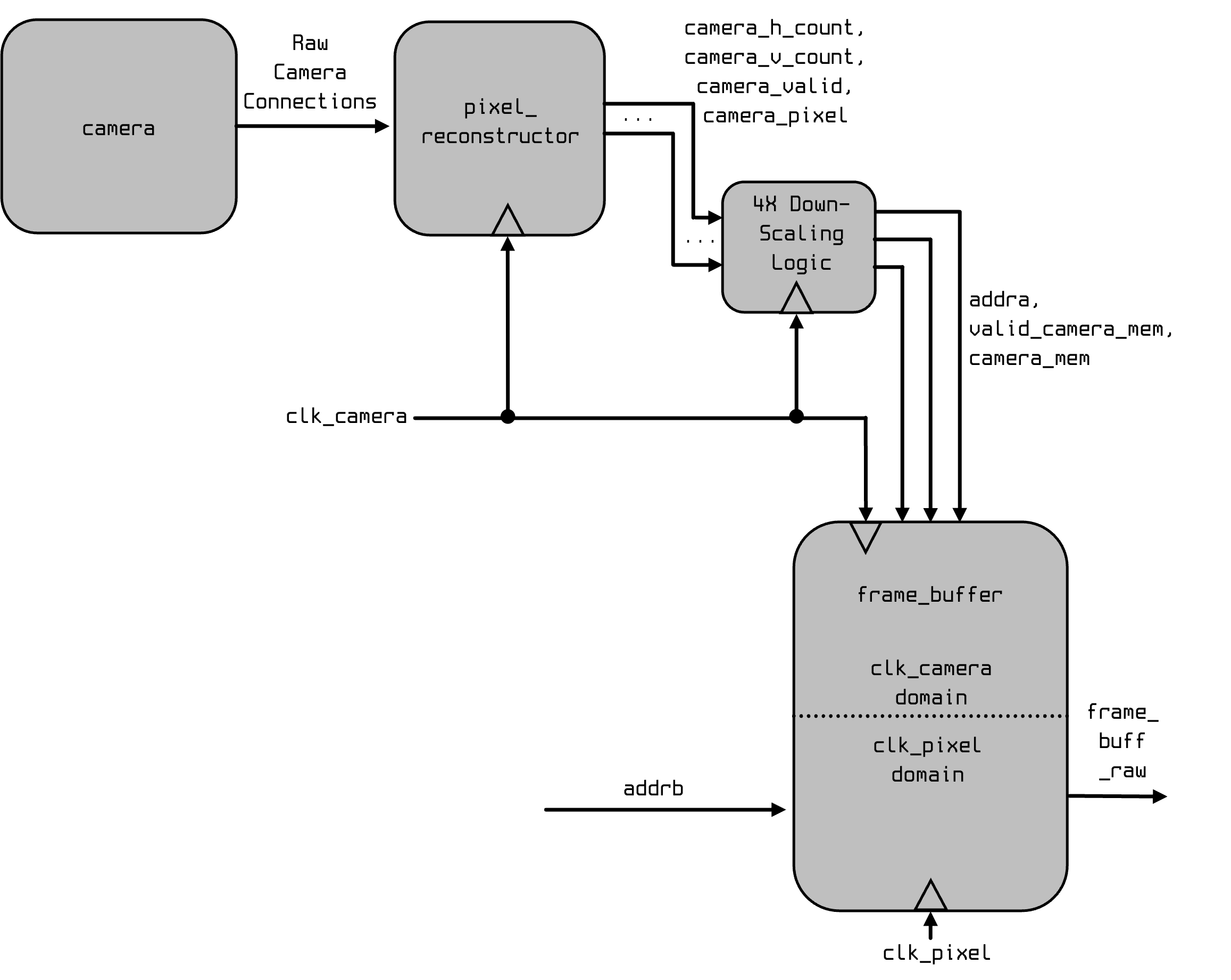
Now we're doing this:

New Parts

CDC

In this new design, we want to do our convolution not on the 200 MHz camera clock but on our slower 74.25 MHz HDMI clock (clk_pixel). Annoyingly, in our previous design, that clock domain crossing didn't happen until the frame buffer and we need to do our convolution before that. The solution is to do clock domain crossing earlier. To do that we'll use a fifo made using a Vivado Parameterized Macro. This is effectively a small BRAM FIFO that will move us without any warnings from 200 MHz to 74.25 MHz. Since the camera is only sending in data (worst case) every fourth clock cycle and likely every eighth, we should be totally fine moving from 200 MHz to 74.25 MHz and run into no data build-up issues (note for final projects to always think about this! FIFOs only take care of short term data mismatches and not long-term over-production mismatch situations in a design).

Filter 0

After this we have our first filter. This is a 3x3 Gaussian Blur filter that will be used to do some anti-aliasing protection (see lecture 12). We'll talk about the filter design in a minute.

Downsampling

After that we're going to use a Line buffer (also discussed below) to temporarily hold a few lines of our image in storage for the benefit of downstream filters. The logic used to write to this line buffer is identical to what you wrote in Lab 05 for down-sampling into the original frame_buffer. We'd use a full frame buffer here if we had infinite resources, but a line buffer will do.

Note it is "better" to downsample like we do now since we've already run it through our anti-aliasing filter (the first Gaussian Blur).

Filters and Selection

After the down-sampling and the storage, we'll then feed the output into a number of different filters (again we'll talk about the filters below). After that is a multiplexer which chooses among them is passed on to the actual full frame_buffer for display. Note the frame buffer now is on a single clock domain since we did the crossing (and sub-sampling) earlier in our pipeline.

Switch Reference

All of the switches and user controls are described here in summary:

• btn[2] still programs/reprograms the camera. Refer back to the camera usage instructions in lab 5.
• btn[1] controls whether or not the first layer of filtering (gaussian blur) happens or not: (this will let us see some aliasing)
  • unpushed it does
  • pushed it does not (bypass useful for testing line buffer)
• sw[2:0] controls which filters are active in the pipeline:
  • 000 Identity Kernel
  • 001 Gaussian Blur
  • 010 Sharpen
  • 011 Ridge Detection
  • 100 Sobel Y-axis Edge Detection
  • 101 Sobel X-axis Edge Detection
  • 110 Total Sobel Edge Detection
  • 111 Output of Line Buffer Directly (Helpful for debugging line buffer in first part)
• sw[4:3] controls the color channel used to produce our mask, where (we'll just do y cr cb since they're better)
  • 00 Y channel
  • 01 Cr channel
  • 10 Cb channel
  • 11 no output
• sw[6:5] controls how the color mask is displayed, where:
  • 00 shows raw camera output
  • 01 shows the color channel being used to produce the mask. For example, if the blue channel was selected with sw[5:3]=010, then we'd output the 12-bit color {b, b, b} to the screen.
  • 10 displays the mask itself
  • 11 turns the mask pink, and overlays it against a greyscale'd camera output.
• sw[7] controls what's done with the CoM information:
  • 0 nothing
  • 1 crosshair
• sw[11:8] set the lower bound on our mask generation.
• sw[15:12] set the upper bound on our mask generation.

The Filter

Your big task in this lab is to build the image filter. The code for it is provided to you and doesn't need to get changed.

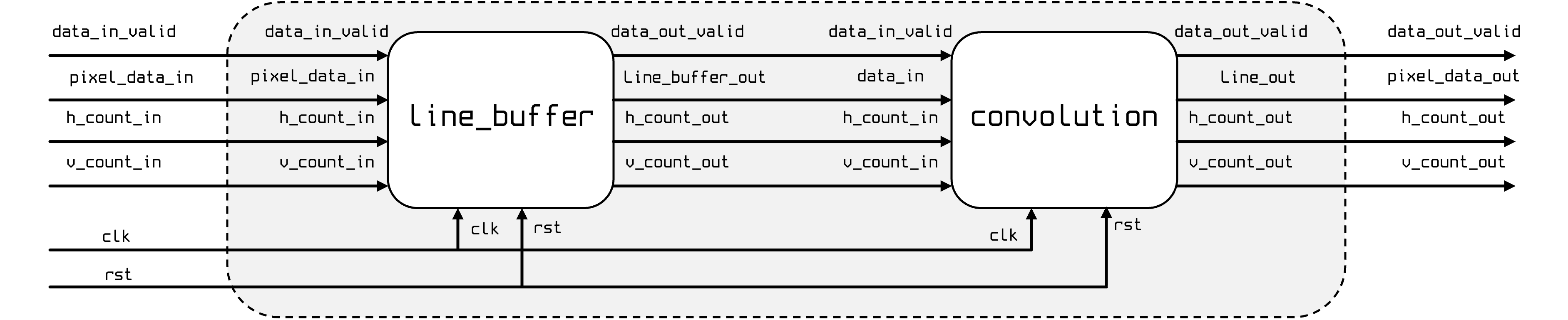
It is comprised of two modules, that you do need to build, though.

• The line_buffer module which is a series of rolling line buffers that give ready access to the n\times n required pixels of a n-kernel.
• The convolution module which performs convolution and maintains an internal n\times n cache of pixels.

For the purposes of this lab, we'll just be building 3x3 filters (this will be difficult enough), but the same idea can be expanded to arbitrarily high dimensions (with proper pipelining, so our combinational paths don't get prohibitively long).

Now let's talk about both portions.

Line Buffer

To start this design, we're going to work on the line_buffer module.

Performing convolution requires us to access multiple pixel values in the input image to produce one pixel in the output image. For the 3x3 kernels we use in this lab, we'll need to access 9 pixels at a given time. This is new requirement for our system! So far we've only needed one pixel at any given time, so we'll have to be clever here. We have a few options for how to do this:

• The simplest approach is to make 9 identical BRAMs, and offset the data in each so that we get 9 pixels on each clock cycle. This wouldn't actually fit on the FGPA - our 320x180 framebuffer takes up between 25% and 50% of the block memory onboard the FPGA as it is, so 8 more of those is probably not going to work.

• We could just read out from our existing framebuffer really really fast. It'd be lovely if we could read 9 pixels out of our framebuffer in one 74.25MHz clock cycle - but that requires a 668.25 MHz clock that we'd have to synchronize with the rest of our system. That's too fast for our FPGA, and we don't want to have to deal with even more clock domain crossing. And if we wanted an even larger kernel, we'd need an even more impossible clock. We can do better.

The solution we'll be rolling with is a rolling line buffer.¹ When a line of data comes off the camera (or any source of pixels accompanied by h_count and v_count information for that matter), we'll read it into one BRAM in a bank of N+1 BRAMs, which each store a horizontal line from the camera. We'll read out from N of these BRAMs into a small NxN cache, which stores the last N values from each line. This works because convolution requires us to scan through our image, which our camera's output is already making us do anyways. The figures do a good job showing how this works:

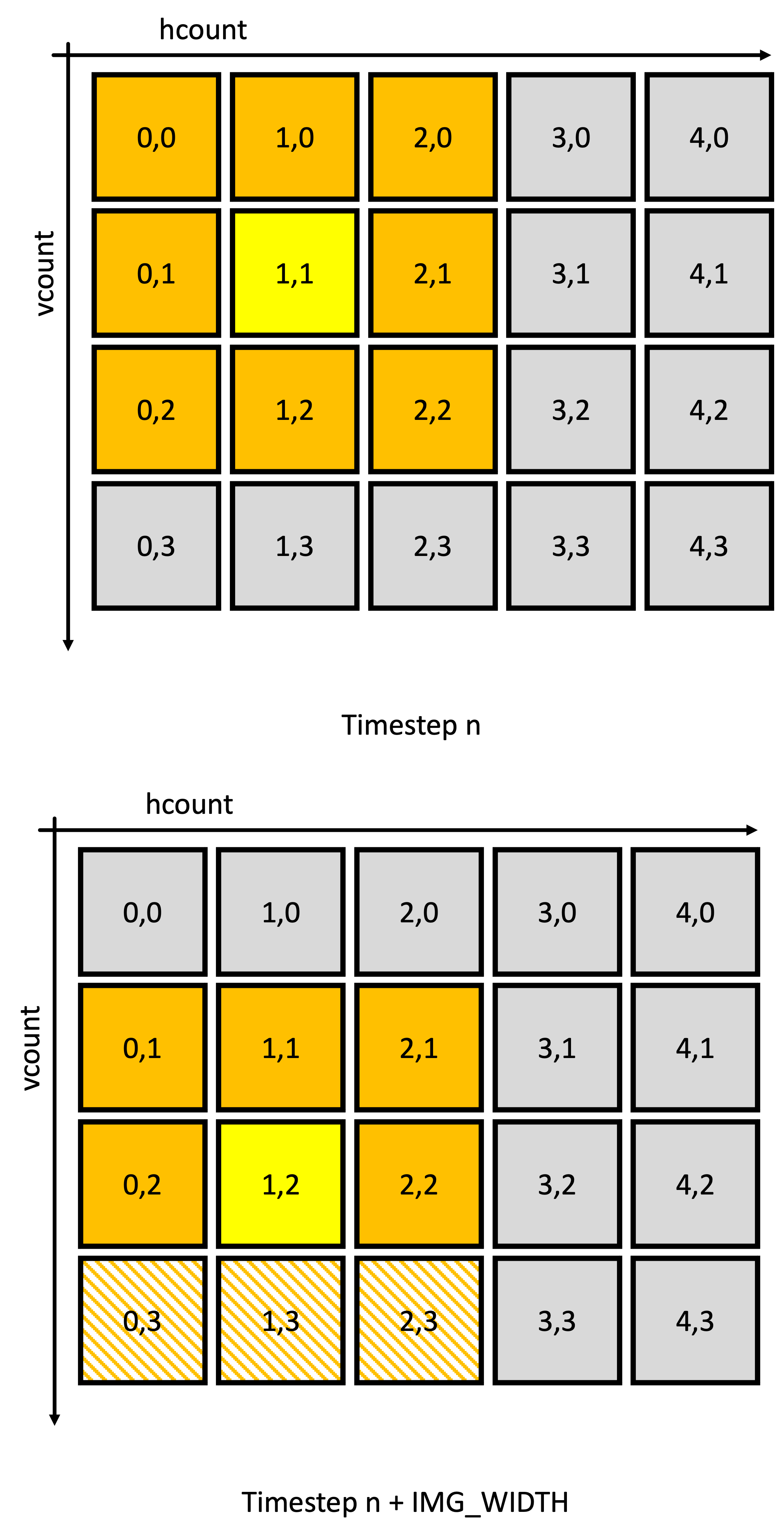
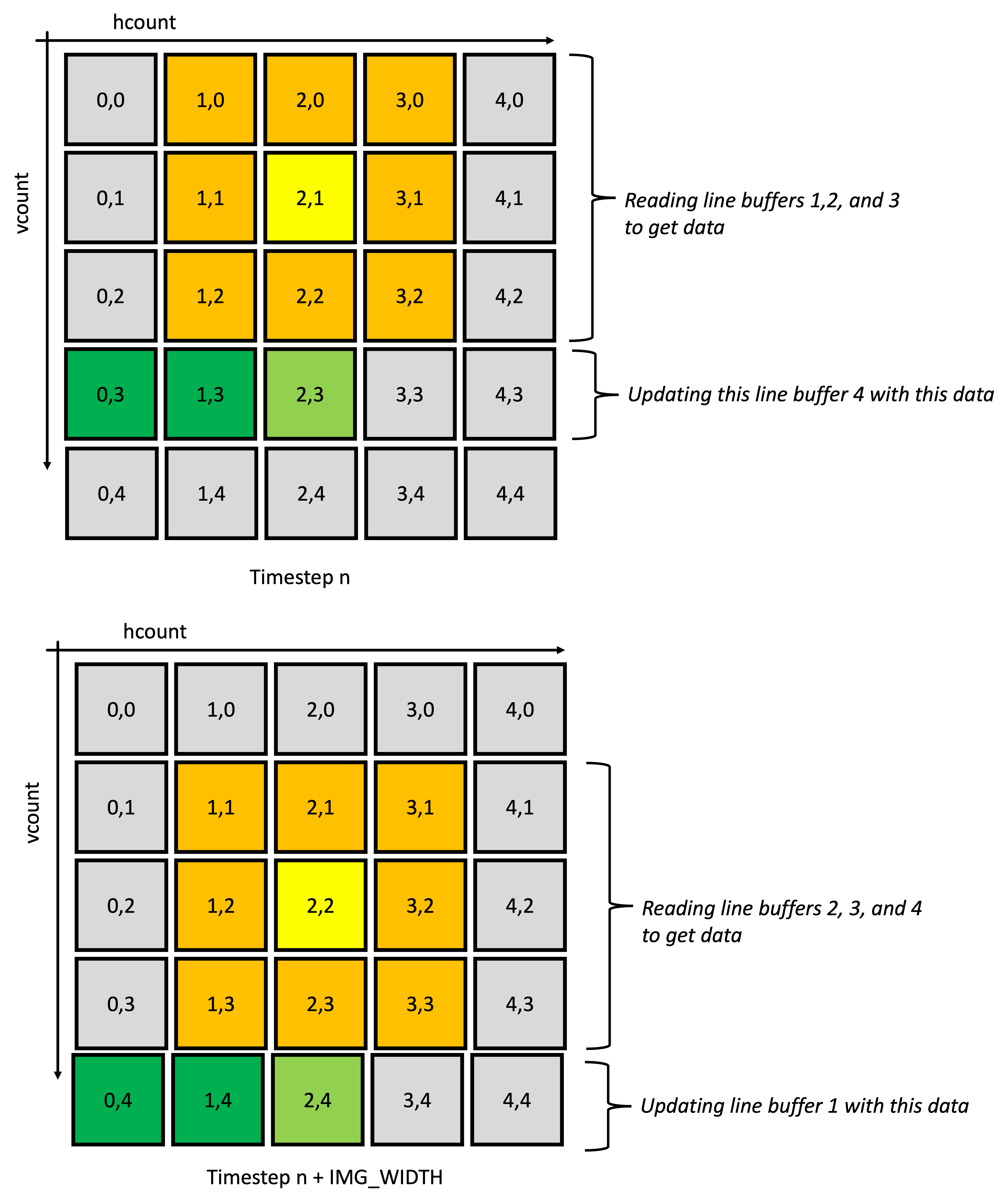
In conclusion: to carry out convolution on one pixel of the image per clock cycle, we only need to introduce in one new pixel per line, per clock cycle. We'll need to buffer three lines for our 3x3 kernel, which will require instantiating four BRAMs.

We're going to split the storage of the 3x3 grid of pixels across two modules. The line_buffer module will output the pixel at the current h_count from the previous three lines, which get handed off to the convolution module. The convolution module will use these to assemble a 3x3 cache of pixels, which it'll then use for math we do with the kernel.

Let's turn to writing the line_buffer module, which has the following inputs and outputs:

module line_buffer (
            input wire clk, //system clock
            input wire rst, //system reset

            input wire [10:0] h_count_in, //current h_count being read
            input wire [9:0] v_count_in, //current v_count being read
            input wire [15:0] pixel_data_in, //incoming pixel
            input wire data_in_valid, //incoming  valid data signal

            output logic [KERNEL_DIMENSION-1:0][15:0] line_buffer_out, //output pixels of data
            output logic [10:0] h_count_out, //current h_count being read
            output logic [9:0] v_count_out, //current v_count being read
            output logic data_out_valid //valid data out signal
  );
  parameter HRES = 1280;
  parameter VRES = 720;

  localparam KERNEL_DIMENSION = 3;
endmodule

The primary job of the buffer is to output the value of the pixel at h_count_in from the previous three lines, and store the pixel provided to it in the current line. More explicitly, it should set:

• line_buffer_out[0] = the pixel at (h_count, v_count-3)
• line_buffer_out[1] = the pixel at (h_count, v_count-2)
• line_buffer_out[2] = the pixel at (h_count, v_count-1)
• …and save the value of the pixel at (h_count, v_count)

You’ll do this by making four BRAMs, and muxing between them to produce line_buffer[2:0]. You’ll direct the value of the newest pixel at (h_count_in, v_count_in) to be written to one BRAM, and you’ll direct the output of the remaining three BRAMs to line_buffer_out. You’ll need to pay particular attention to which BRAM’s output gets muxed to which index in line_buffer_out, as once a new line occurs the BRAM containing the line at v_count-1 will contain the line at v_count-2. You’ll have to make sure each BRAM rolls over into it’s proper location in line_buffer_out.

A few details for how to do this:

• Since we’re working images of a variety of sizes (1280x720, 320x180, etc...) each BRAM should be of a parameterized length (the HRES) parameter. The HRES parameter will be useful in knowing when to wrap around our line buffer cycling.
• Our camera outputs pixels with 565 encoding, and you can just assume we'll only be working with 565 16 bit color, so we’ll need to store values that are 16 bits wide. Use a few instances of our creatively-named friend xilinx_true_dual_port_read_first_1_clock_ram for this. An example instantiation is provided in the file, but we strongly encourage a generate loop structure like can be found in the top_level provided.
• Each BRAM should be addressed at the same location, since we're considering the pixel at the same h_count for all four.
• You should control which BRAM is being written to and which are being read from by changing the value on their wea ports.
• We’ll only pull pixels into our buffer when data_in_valid is asserted. If it's not asserted, then the location of (h_count, v_count) isn't inside our camera image and we don't want to save those pixels.
• We’ll need to pipeline our outputs. Each BRAM takes two clock cycles to read from, so we should compensate by adding two clock cycles of delay between data_in_valid and data_out_valid. Furthermore, if v_count_in is a value n, have v_count_out be a value (n-2) \mod VRES since the three pixels being read out are centered two lines behind the newest line being read in. This should go without saying at this point, but absolutely do not use the modulo operator % for this - that generates a lot of logic that we don't need and will break timing! Just use an if/else if/else statment here to handle the troublesome cases.

Develop this module in simulation using a testbench! You pretty much have to since there's no easy way to check your early results in hardware. A good simulation to create would be one that:

• Mimics the expected h_count and v_count pattern of our image.
• Tests that pixels are only written to memory when data_in_valid is asserted.
• Verifies that data_out_valid goes high two cycles after data_in_valid does.
• Verifies that when the pixel info for (h_count and v_count) is being written in that the pixel info for (h_count,v_count-3), (h_count,v_count-2), and (h_count,v_count-1) is being read out with the expected two clock-cycle latency. To do this you'll need to clock in differing pixel values on each line - otherwise you won't be able to tell what values your buffer's pulling!

When you are confident your design is close in simulation, then you can test it on the board by seeing if you can regular video through. If you study the top_level.sv and the diagram we provided earlier, in addition to the line_buffer getting used in the filter we also use an instance of it (in conjunction with some 4x4 down-sample logic) to hold values prior to feeding them into the second layer of filters.

If you:

• hold btn[1] to bypass your currently non-functioning filter0 and...
• make sure sw[2:0] are set to 7 to bypass all second layer filters...

You should be able to see a regular video feed on your display. If not, then there is likely an issue with your line buffer. So back to simulation and debugging.

For checkoff 1 below, be prepared to show your line buffer working in simulation. If you don't have that done, then you will not get the checkoff and we'll remove you from the queu until you do have it.

Checkoff 1:
Show us your line_buffer module working in simulation and demonstrate the line_buffer being used to pass through data to the down sampling logic in the top level.

Loading...

Convolution

The next step is the convolution module. This module maintains its own internal 3x3 cache that's updated from the line_buffer, and this nine pixel cache is what the actual convolution is done on. The actual convolution is conceptually pretty straightforward (it's just multiplying and adding) but the implementation is rather nuanced because we'll have to deal with fractions and signed numbers. Let's talk about this.

When you need to multiply by a fraction in low-level digital design, you can't just do it directly since there's no way to have actual fractional values. All we have are bits and the bits are indivisible. The workaround is to do the top part as multiplication and then the bottom part as division. You need to make sure to do the multiplication first and then the division since if you do it in the other way, you'll potentially lose bits of information.

In this lab, we'll need to do basically this for the kernels (like the Gaussian) that have fractional values. We'll need to keep track of both our kernel coefficients as well as the amount to shift by at the very end. This requires a fair number of parameters and it's a lot to keep track of, and since kindness is a virtue, we've defined all of the kernel coefficients and bit shifts for you in the kernels.sv provided for you. Have a look inside the file, you'll instantiate a copy of the kernels module to hold all the values.

Further complicating things is that some kernels have entries with negative values - and are designed to make output pixels that can be negative. These aren't displayable, so if we get a negative number from our convolution math, we'll want to just output zero instead.

Further further compliating things, it is possible with some kernels to get a result that is larger than what can be held in our pixel (5 bits in the case of blue and red and 6 bits in the case of green). You may find you need to clip your final result here as well (at 31 and 63 for red/blue and green, respectively, however I've found this is far less of a problem than the signed math issues and the underflow negative results issue).

Since there's so much math happening here, doing it all at once with combinational logic will likely² break timing. We've found that you'll need to spread the sequence of multiply/add/shift/negative check over at least two clock cycles. If you don't do this your simulation will still work (it doesn't know about the timing constraints on our particular chip) but you'll get negative slack in your built design. You can check this by searching through the build log for the WNS value and making sure it isn't negative. Make sure you're checking the last reported value of WNS in the vivado.log file - Vivado does a few stages of optimization on your design to meet timing, and it throws out the WNS value at each stage. To pass the lab, you need positive WNS.

Signed Math

Just one more thing before we jump into Verilog. We're performing signed math here, which requires that Verilog interpret the values of every term in our multiplication/addition/shift as signed. This is fine and dandy, but we need to keep a few things in mind:

• The result of any part select (the square brackets foo[a:b] that let us pull bits out of larger arrays) is automatically considered unsigned. This means that when you pull RGB values out of a 16-bit pixel value, you'll need to tell Verilog to interpret the result as a signed number. You should do this with the $signed(x) function, which returns a version of x interpreted as a signed number. Be careful though, this function will interpret whatever you give it with two's complement logic, so make sure you pad your value with an extra zero so the MSB of your value doesn't get mistaken for the sign bit. Something like $signed({1'b0, foo[a:b]}) should do nicely.
• Similarly, we'll also have to make our bitshifts respect the sign of our numbers. Use the triple shift >>> for this, as it copies over the sign bit into the output.

Let's finally turn to implementing convolution, which we've provided a skeleton for in convolution.sv. Just to be super explicit about what we're asking you to do:

• Maintain a 3x3 cache of pixel values, which clocks in new pixel values from the line buffer when data_in_valid is asserted.
• For each color channel, multiply each entry in the 3x3 cache by the appropriate entry in the kernel.
• Shift this value by the appropriate amount for the given kernel (many have no shift keep in mind).
• If this value is negative, output zero instead.
• If this value is greater than the capacity of the color channel, clip it at the max value.
• Be properly pipelined. You'll need a few clock cycles to do your math, so make sure to pipeline the data_valid, h_count, and v_count signals appropriately. I think I did mine in two cycles.
• I'll say this again, even with the sinfully luxurious 13.4ns our 74.25 MHz clock affords us, there is no way you'll do all this math in one clock cycle and manage to close timing. If you put yourself on the queue, and are saying "why no work?" to me and it turns out you're trying to do the entire thing in one clock cycle, I'll....well I won't be mad, but I'll be disappointed... Just don't do it. Spread your math out over some cycles...as long as the accompanying metadata of h_count and v_count and data_out_valid are pipelined a identical amount, nobody except you and your god will know that you took 26.8 ns to convolve rather than 13.4 ns.

Testbench

Do not try to write convolution without testbenching. It will be a nightmare. Start with very simple input kernels since their results should be easy to calculate and verify by hand. Then go from there. Make sure you've tested signed math with some of the kernels with negatives! Look out for underflow, usually indicative of a sign misinterpretation somewhere.

Only when you feel good with your results should you move to your real-life system.

from PIL import Image

im_input = Image.open("filename.png")
im_input = im.convert('RGB')
# example access pixel at coordinate x,y
pixel = im_input.getpixel( (x,y) )
# pixel is a tuple of values (R,G,B) ranging from 0 to 255

# create a blank image with dimensions (w,h)
im_output = Image.new('RGB',(w,h))
# write RGB values (r,g,b) [range 0-255] to coordinate (x,y)
im_output.putpixel((x,y),(r,g,b))
# save image to a file
im_output.save('output.png','PNG')

Testbenching with Vivado (Vicoco)

So far whenever we've run our testbenches, we've run our Python/cocotb code with Icarus (iVerilog) as our simulator--but as some of you may have already discovered, Icarus isn't always guaranteed to behave the same way as Vivado when we synthesize our designs for the FPGA; some formats of logic indexing may have given you a Sorry ... message that indicates you may have encountered this. The differences between Icarus and Vivado when it comes to signed math are more severe. However, Vivado has a simulator built-in, that should⁴ behave the same as our synthesized design in terms of interpreting signed math. So, we want to use the Vivado simulator to test our convolution design, and be able to catch signed-math errors in simulation!

Cocotb natively has support for switching between several simulators as the backend, but unfortunately none of those simulators are Vivado's simulator. In order to use the Vivado simulator, we'll need to utilize an additional package, vicoco; it's an EXPERIMENTAL add-on to cocotb that lets you use the Vivado simulator insead of Icarus when running your testbench⁵. For the 90% of you that don't have Vivado installed locally, we also have lab-bc set up to let you run Vivado/Vicoco simulations through the lab machines so that you get your waveforms back! Go take a look at the documentation page to get vicoco installed on your machine. You need it to be able to reliably test your signed math, so go install it!

Errors

This thing, when working incorrectly, can make some weird looking errors. You should appreciate them, but them being cool should not be mistaken with them working.

Now how is it supposed to work? Here's my system working in my dump of an office as I flip through all the kernels. Note the Gaussian blur is the easiest to get working since it is all positive numbers. The ones that tend to cause issues are the other kernels that have negatives involved.

Here's a video of a bad version (with a couple mistakes related to signed numbers and thresholding). Notice how the blur looks perfectly fine (there's no negatives involved in that kernel). A obvious tell of signed issues is how on the Sobel X and Sobel Y, the X and Y features, respectively are being found, but the regions that should be black have very bright RGB speckling. This is likely arising from either a signed number issue or a negative getting treated as a positive or poor low-side clipping, etc... All of these errors can look similar so be on the lookout. The effect looks admittedly cool, but it is not what we want (Feel free to save the bit files though and listen to some Jefferson Airplane (remember what the dormouse...feed your head) while looking at them later on.). It needs to be fixed for the actual checkoff.

Checkoff 2:

Show us your convolutional module working in simulation. In addition, have your buffer and convolution modules working in hardware. We'll want to see:

• The WNS of your design. Be sure it's positive!
• Your convolution module working in simulation.
• Your convolution and buffer modules working together in hardware, and applying kernels selectable by sw[2:0]
• Working grating tracking using the X and Y edge detection filters described above.

Loading...

Zip up and upload your hdl folder (all files) here.

Select File No file selected

Loading...

Zip up and upload your testbenches for both line_buffer and convolution here.

Select File No file selected

Loading...